SHEERO Guide

Introduction
This is an example of the workflow a SHEERO study site might use to add geomarkers to their data with DeGAUSS.
If you have used DeGAUSS, would you mind providing us some feedback and completing a short survey?
Overview:
Steps 0 through 2: Install Software and Prepare Data
Steps 3 through 7: Use DeGAUSS to geocode addresses add geomarkers (columns added in each step are highlighted in gray). Note that in each step, the input file is the CSV created in the previous step.
Step 8: Link to Census Data
Step 9: Use DeGAUSS to add daily air pollution data.
Step 10: Remove PHI before sharing.
Step 0: Install Docker
See the Installing Docker webpage.
Note about Docker Settings:
After installing Docker, but before running containers, go to Docker Settings > Advanced and change memory to greater than 4000 MB (or 4 GiB)
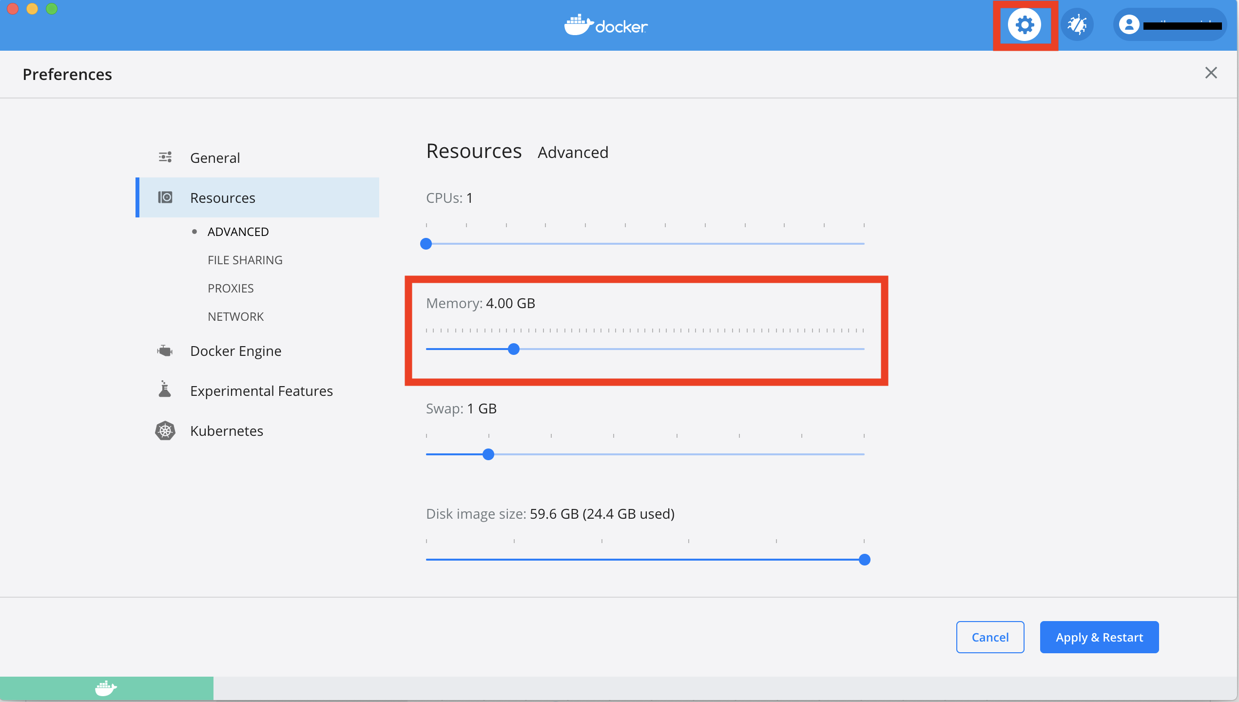
If you are using a Windows computer, also set CPUs to 1.
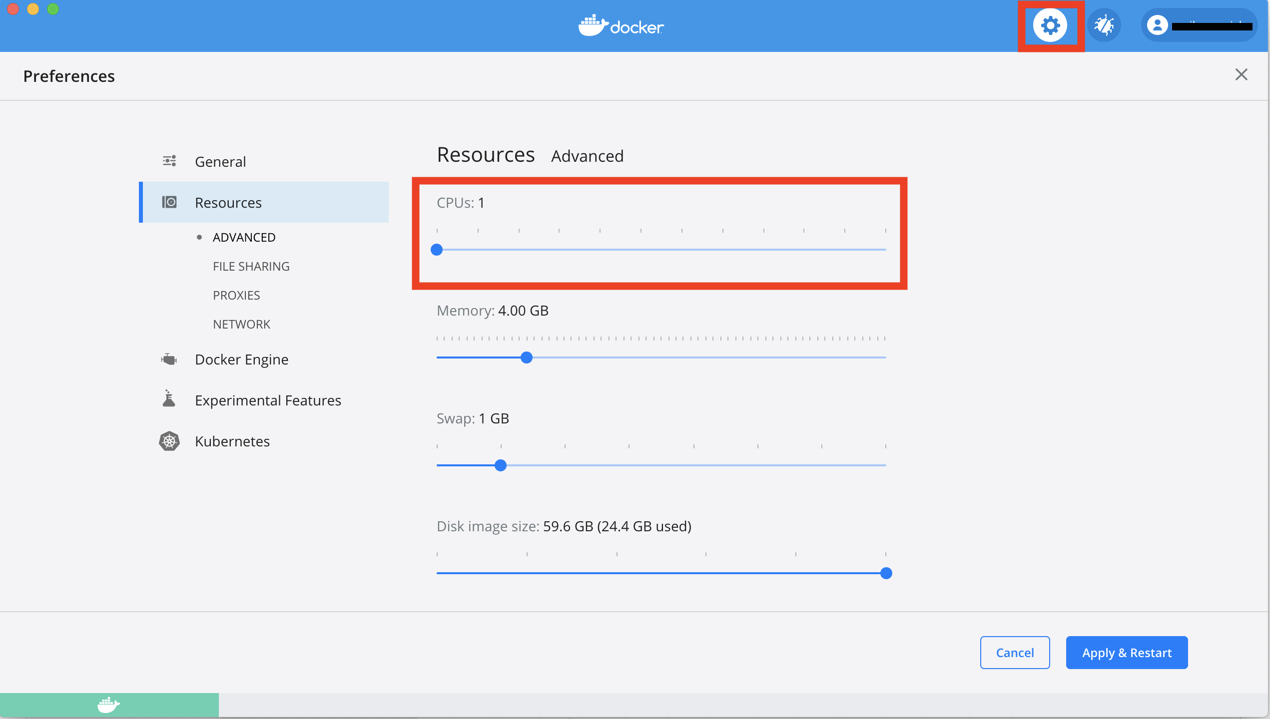
Click Apply and wait for Docker to restart.
Step 1: Preparing Your Input File
The input file must be a CSV file with one column called
address containing all address components. Other columns
may be present and will be returned in the output file, but should be
kept to a minimum to reduce file size.
An example input CSV file (called my_address_file.csv)
might look like:
| id | address |
|---|---|
| 13100070229 | 1922 CATALINA AV CINCINNATI, OH 45237 |
| 54000600136 | 5358 LILIBET CT DELHI TOWNSHIP, OH 45238 |
| 11200020024 | 630 GREENWOOD AV CINCINNATI, OH 45229 |
Refer to the DeGAUSS geocoding webpage for more information about the input file and address string formatting.
Working with home and school addresses
Because the geocoder requires one address column named
address, we suggest that home addresses and school
addresses be stored in separate CSV files and geocoded separately. This
means that steps 3 through 10 will be done twice– once for home
addresses and once for school addresses. Alternatively, home and school
addresses can be in the same file in long format (i.e., with a column
that defines the type of address as home or
school and one column that contains the
address).
Step 3: Geocoding
After navigating to your working directory, use the ghcr.io/degauss-org/geocoder
to geocode your addresses.
macOS example call:
docker run --rm -v "$PWD":/tmp ghcr.io/degauss-org/geocoder:3.2.0 my_address_file.csvReplace my_address_file.csv with the name of the CSV
file to be geocoded and run the call in the shell.
Note for Windows Users:
In this and all following docker calls in this example, replace"$PWD"with"%cd%". Refer to the DeGAUSS Troubleshooting page for more information.
See here for more information on the anatomy of a degauss command.
The output file is written to the same directory and
in our example, will be called
my_address_file_geocoded_3.2.0.csv.
Example output:
| id | address | start_date | end_date | matched_street | matched_zip | matched_city | matched_state | lat | lon | score | precision | geocode_result |
|---|---|---|---|---|---|---|---|---|---|---|---|---|
| 54000600136 | 5358 LILIBET CT DELHI TOWNSHIP OH 45238 | 2015-05-05 | 2015-05-06 | Lilibet Ct | 45238 | Delhi Hills | OH | 39.11552 | -84.61902 | 0.754 | range | geocoded |
| 13100070229 | 1922 CATALINA AV CINCINNATI OH 45237 | 2010-06-07 | 2010-06-08 | Catalina Ave | 45237 | Cincinnati | OH | 39.17112 | -84.46176 | 0.922 | range | geocoded |
| 11200020024 | 630 GREENWOOD AV CINCINNATI OH 45229 | 2019-07-08 | 2019-07-09 | Greenwood Ave | 45229 | Cincinnati | OH | 39.15321 | -84.49236 | 0.922 | range | geocoded |
For more information on interpreting geocoder output, see here.
Step 4: Census Block Group
macOS example call:
docker run --rm -v "$PWD":/tmp ghcr.io/degauss-org/census_block_group:0.5.1 my_address_file_geocoded_3.2.0.csv 2010Replace my_address_file_geocoded_3.2.0.csv with the name
of the geocoded CSV file created in Step 3 and run.
Note: The CCAAPS cohort should repeat this step,
replacing 2010 with 2000, resulting in a file
with both 2010 census identifiers and 2000 census
identifiers.
The output file is written to the same directory
and, in our example, will be called
my_address_file_geocoded_3.2.0_census_block_group_0.5.1_2010.csv.
Example output:
| id | address | matched_street | matched_zip | matched_city | matched_state | lat | lon | score | precision | geocode_result | fips_block_group_id_2010 | fips_tract_id_2010 |
|---|---|---|---|---|---|---|---|---|---|---|---|---|
| 54000600136 | 5358 LILIBET CT DELHI TOWNSHIP OH 45238 | Lilibet Ct | 45238 | Delhi Hills | OH | 39.11552 | -84.61902 | 0.754 | range | geocoded | 390610213032 | 39061021303 |
| 13100070229 | 1922 CATALINA AV CINCINNATI OH 45237 | Catalina Ave | 45237 | Cincinnati | OH | 39.17112 | -84.46176 | 0.922 | range | geocoded | 390610063004 | 39061006300 |
| 11200020024 | 630 GREENWOOD AV CINCINNATI OH 45229 | Greenwood Ave | 45229 | Cincinnati | OH | 39.15321 | -84.49236 | 0.922 | range | geocoded | 390610068003 | 39061006800 |
More information on the census_block_group container
Step 5: Average Annual Daily Traffic
macOS example call:
docker run --rm -v "$PWD":/tmp ghcr.io/degauss-org/aadt:0.2.0 my_address_file_geocoded_3.2.0_census_block_group_0.5.1_2010.csv Replace
my_address_file_geocoded_3.2.0_census_block_group_0.5.1_2010.csv
with the name of the CSV file created in Step 4 and run.
The output file is written to the same directory and
in our example, will be called
my_address_file_geocoded_3.2.0_census_block_group_0.5.1_2010_aadt_0.2.0_400m_buffer.csv.
Example output:
| id | address | matched_street | matched_zip | matched_city | matched_state | lat | lon | score | precision | geocode_result | fips_block_group_id_2010 | fips_tract_id_2010 | length_stop_go | length_moving | vehicle_meters_stop_go | vehicle_meters_moving | truck_meters_stop_go | truck_meters_moving |
|---|---|---|---|---|---|---|---|---|---|---|---|---|---|---|---|---|---|---|
| 54000600136 | 5358 LILIBET CT DELHI TOWNSHIP OH 45238 | Lilibet Ct | 45238 | Delhi Hills | OH | 39.11552 | -84.61902 | 0.754 | range | geocoded | 390610213032 | 39061021303 | 900 | 0 | 12120535 | 0 | 0 | 0 |
| 13100070229 | 1922 CATALINA AV CINCINNATI OH 45237 | Catalina Ave | 45237 | Cincinnati | OH | 39.17112 | -84.46176 | 0.922 | range | geocoded | 390610063004 | 39061006300 | 350 | 0 | 2098249 | 0 | 0 | 0 |
| 11200020024 | 630 GREENWOOD AV CINCINNATI OH 45229 | Greenwood Ave | 45229 | Cincinnati | OH | 39.15321 | -84.49236 | 0.922 | range | geocoded | 390610068003 | 39061006800 | 0 | 0 | 0 | 0 | 0 | 0 |
More information on aadt
Step 6: Distance to Roadway
macOS example call:
docker run --rm -v "$PWD":/tmp ghcr.io/degauss-org/roads:0.2.1 my_address_file_geocoded_3.2.0_census_block_group_0.5.1_2010_aadt_0.2.0_400m_buffer.csvReplace
my_address_file_geocoded_3.2.0_census_block_group_0.5.1_2010_aadt_0.2.0_400m_buffer.csv
with the name of the CSV file created in Step 5 and run.
The output file is written to the same directory and
in our example, will be called
my_address_file_geocoded_3.2.0_census_block_group_0.5.1_2010_aadt_0.2.0_400m_buffer_roads_0.2.1_400m_buffer.csv.
Example output:
| id | address | matched_street | matched_zip | matched_city | matched_state | lat | lon | score | precision | geocode_result | fips_block_group_id_2010 | fips_tract_id_2010 | length_stop_go | length_moving | vehicle_meters_stop_go | vehicle_meters_moving | truck_meters_stop_go | truck_meters_moving | dist_to_1100 | dist_to_1200 | length_1100 | length_1200 |
|---|---|---|---|---|---|---|---|---|---|---|---|---|---|---|---|---|---|---|---|---|---|---|
| 54000600136 | 5358 LILIBET CT DELHI TOWNSHIP OH 45238 | Lilibet Ct | 45238 | Delhi Hills | OH | 39.11552 | -84.61902 | 0.754 | range | geocoded | 390610213032 | 39061021303 | 900 | 0 | 12120535 | 0 | 0 | 0 | 15436 | 165399 | 0 | 0 |
| 13100070229 | 1922 CATALINA AV CINCINNATI OH 45237 | Catalina Ave | 45237 | Cincinnati | OH | 39.17112 | -84.46176 | 0.922 | range | geocoded | 390610063004 | 39061006300 | 350 | 0 | 2098249 | 0 | 0 | 0 | 6143 | 165509 | 0 | 0 |
| 11200020024 | 630 GREENWOOD AV CINCINNATI OH 45229 | Greenwood Ave | 45229 | Cincinnati | OH | 39.15321 | -84.49236 | 0.922 | range | geocoded | 390610068003 | 39061006800 | 0 | 0 | 0 | 0 | 0 | 0 | 7532 | 165509 | 0 | 0 |
More information on roads
Step 7: Greenspace
macOS example call:
docker run --rm -v "$PWD":/tmp ghcr.io/degauss-org/greenspace:0.3.0 my_address_file_geocoded_3.2.0_census_block_group_0.5.1_2010_aadt_0.2.0_400m_buffer_roads_0.2.1_400m_buffer.csvReplace
my_address_file_geocoded_3.2.0_census_block_group_0.5.1_2010_aadt_0.2.0_400m_buffer_roads_0.2.1_400m_buffer.csv
with the name of the CSV file created in Step 6 and run.
The output file is written to the same directory and
in our example, will be called
my_address_file_geocoded_3.2.0_census_block_group_0.5.1_2010_aadt_0.2.0_400m_buffer_roads_0.2.1_400m_buffer_greenspace_0.3.0.csv.
Example output:
| id | address | matched_street | matched_zip | matched_city | matched_state | lat | lon | score | precision | geocode_result | fips_block_group_id_2010 | fips_tract_id_2010 | length_stop_go | length_moving | vehicle_meters_stop_go | vehicle_meters_moving | truck_meters_stop_go | truck_meters_moving | dist_to_1100 | dist_to_1200 | length_1100 | length_1200 | evi_500 | evi_1500 | evi_2500 |
|---|---|---|---|---|---|---|---|---|---|---|---|---|---|---|---|---|---|---|---|---|---|---|---|---|---|
| 54000600136 | 5358 LILIBET CT DELHI TOWNSHIP OH 45238 | Lilibet Ct | 45238 | Delhi Hills | OH | 39.11552 | -84.61902 | 0.754 | range | geocoded | 390610213032 | 39061021303 | 900 | 0 | 12120535 | 0 | 0 | 0 | 15436 | 165399 | 0 | 0 | 0.4182615 | 0.4350124 | 0.4295556 |
| 13100070229 | 1922 CATALINA AV CINCINNATI OH 45237 | Catalina Ave | 45237 | Cincinnati | OH | 39.17112 | -84.46176 | 0.922 | range | geocoded | 390610063004 | 39061006300 | 350 | 0 | 2098249 | 0 | 0 | 0 | 6143 | 165509 | 0 | 0 | 0.3356100 | 0.3556324 | 0.3863916 |
| 11200020024 | 630 GREENWOOD AV CINCINNATI OH 45229 | Greenwood Ave | 45229 | Cincinnati | OH | 39.15321 | -84.49236 | 0.922 | range | geocoded | 390610068003 | 39061006800 | 0 | 0 | 0 | 0 | 0 | 0 | 7532 | 165509 | 0 | 0 | 0.4157077 | 0.4082887 | 0.3774101 |
More information on greenspace
Step 8: Census Data
Using the software of your choice, join the census data file to the
file created in Step 7 using the fips_tract_id_2010 column.
If you are unfamiliar with merging data, try following this introduction
in Excel.
Note that any CSV opened in Microsoft Excel will not show leading
zeros. If a CSV is opened in Excel then saved, the leading zeros will be
truncated (e.g., 01234567891 will become
1234567891).
Step 9: Air Pollution
For this simplicity, we suggest using your original address file
after geocoding (the output of Step 3) for this step. This file must
also included columns called start_date and
end_date. The result of this step will be daily air
pollution estimates in long format. In other words, the output file will
contain one row per day between start_date and
end_date for each individual lat and
lon location. This means that the output file will likely
contain many more rows than the input file, so using identifiers with
this container is useful for merging its output with other sources.
Step 9a: schwartz_grid_lookup
This step finds the nearest grid cell with Schwartz pollutant
estimates for each input lat and lon.
macOS example call:
docker run --rm -v "$PWD":/tmp degauss/schwartz_grid_lookup:0.4.1 my_address_file_geocoded_3.2.0.csvReplace my_address_file_geocoded_3.2.0.csv with the name
of the CSV file created in Step 3 and run.
The output file is written to the same directory and
in our example, will be called
my_address_file_geocoded_3.2.0_schwartz_site_index.csv.
Example output:
| id | address | start_date | end_date | matched_street | matched_zip | matched_city | matched_state | lat | lon | score | precision | geocode_result | site_index | sitecode |
|---|---|---|---|---|---|---|---|---|---|---|---|---|---|---|
| 54000600136 | 5358 LILIBET CT DELHI TOWNSHIP OH 45238 | 2015-05-05 | 2015-05-06 | Lilibet Ct | 45238 | Delhi Hills | OH | 39.11552 | -84.61902 | 0.754 | range | geocoded | 9596220 | 211050625307 |
| 13100070229 | 1922 CATALINA AV CINCINNATI OH 45237 | 2010-06-07 | 2010-06-08 | Catalina Ave | 45237 | Cincinnati | OH | 39.17112 | -84.46176 | 0.922 | range | geocoded | 9614001 | 211050650500 |
| 11200020024 | 630 GREENWOOD AV CINCINNATI OH 45229 | 2019-07-08 | 2019-07-09 | Greenwood Ave | 45229 | Cincinnati | OH | 39.15321 | -84.49236 | 0.922 | range | geocoded | 9609779 | 211050644503 |
More information on schwartz_grid_lookup
Step 9b: schwartz
This step adds daily Schwartz pollutant estimates based on the grid
identifiers added in Step 9a and start_date and
end_date columns.
macOS example call:
docker run --rm -v "$PWD":/tmp degauss/schwartz:0.5.5 my_address_file_geocoded_3.2.0_schwartz_site_index.csvReplace
my_address_file_geocoded_3.2.0_schwartz_site_index.csv with
the name of the CSV file created in Step 9a and
run.
The output file is written to the same directory and
in our example, will be called
my_address_file_geocoded_3.2.0_schwartz_site_index_schwartz_v0.5.5.csv.
Example output:
| id | address | start_date | end_date | matched_street | matched_zip | matched_city | matched_state | lat | lon | score | precision | geocode_result | site_index | sitecode | date | year | gh6 | gh3 | gh3_combined | PM25 | NO2 | O3 |
|---|---|---|---|---|---|---|---|---|---|---|---|---|---|---|---|---|---|---|---|---|---|---|
| 11200020024 | 630 GREENWOOD AV CINCINNATI OH 45229 | 2019-07-08 | 2019-07-09 | Greenwood Ave | 45229 | Cincinnati | OH | 39.15321 | -84.49236 | 0.922 | range | geocoded | 9609779 | 211050644503 | 2019-07-08 | 2019 | NA | NA | NA | NA | NA | NA |
| 11200020024 | 630 GREENWOOD AV CINCINNATI OH 45229 | 2019-07-08 | 2019-07-09 | Greenwood Ave | 45229 | Cincinnati | OH | 39.15321 | -84.49236 | 0.922 | range | geocoded | 9609779 | 211050644503 | 2019-07-09 | 2019 | NA | NA | NA | NA | NA | NA |
| 13100070229 | 1922 CATALINA AV CINCINNATI OH 45237 | 2010-06-07 | 2010-06-08 | Catalina Ave | 45237 | Cincinnati | OH | 39.17112 | -84.46176 | 0.922 | range | geocoded | 9614001 | 211050650500 | 2010-06-07 | 2010 | dngyvg | dng | dng | 5.6 | 19.1 | 47.0 |
| 13100070229 | 1922 CATALINA AV CINCINNATI OH 45237 | 2010-06-07 | 2010-06-08 | Catalina Ave | 45237 | Cincinnati | OH | 39.17112 | -84.46176 | 0.922 | range | geocoded | 9614001 | 211050650500 | 2010-06-08 | 2010 | dngyvg | dng | dng | 12.2 | 22.5 | 50.8 |
| 54000600136 | 5358 LILIBET CT DELHI TOWNSHIP OH 45238 | 2015-05-05 | 2015-05-06 | Lilibet Ct | 45238 | Delhi Hills | OH | 39.11552 | -84.61902 | 0.754 | range | geocoded | 9596220 | 211050625307 | 2015-05-05 | 2015 | dngyd2 | dng | dng | 16.1 | 42.5 | 49.2 |
| 54000600136 | 5358 LILIBET CT DELHI TOWNSHIP OH 45238 | 2015-05-05 | 2015-05-06 | Lilibet Ct | 45238 | Delhi Hills | OH | 39.11552 | -84.61902 | 0.754 | range | geocoded | 9596220 | 211050625307 | 2015-05-06 | 2015 | dngyd2 | dng | dng | 20.8 | 56.5 | 46.9 |
More information on schwartz
(URECA only) Step 9c: pm
Note that the Schwartz model covers the years 2000 - 2016. To obtain
PM\({_2.5}\) estimates beyond 2016,
please use our pm container. If your data ends
before 2016, you can skip this step.
Again, we suggest using your original address file after geocoding
(the output of Step 3) for this step, and your file must also included
columns called start_date and end_date. The
result of this step will be daily air pollution estimates in long
format. In other words, the output file will contain one row per day
between start_date and end_date for each
individual lat and lon location. This means
that the output file will likely contain many more rows than the input
file, so using identifiers with this container is useful for merging its
output with other sources.
macOS example call:
docker run --rm -v "$PWD":/tmp ghcr.io/degauss-org/pm:0.2.0 my_address_file_geocoded_3.2.0.csvReplace my_address_file_geocoded_3.2.0.csv with the name
of the CSV file created in Step 3 and run.
The output file is written to the same directory and
in our example, will be called
my_address_file_geocoded_3.2.0_pm_0.2.0.csv.
Example output:
| id | address | start_date | end_date | matched_street | matched_zip | matched_city | matched_state | lat | lon | score | precision | geocode_result | .row | date | year | h3 | h3_3 | pm_pred | pm_se |
|---|---|---|---|---|---|---|---|---|---|---|---|---|---|---|---|---|---|---|---|
| 54000600136 | 5358 LILIBET CT DELHI TOWNSHIP OH 45238 | 2015-05-05 | 2015-05-06 | Lilibet Ct | 45238 | Delhi Hills | OH | 39.11552 | -84.61902 | 0.754 | range | geocoded | 1 | 2015-05-05 | 2015 | 882a9308a9fffff | 832a93fffffffff | 16.130 | 2.9480 |
| 54000600136 | 5358 LILIBET CT DELHI TOWNSHIP OH 45238 | 2015-05-05 | 2015-05-06 | Lilibet Ct | 45238 | Delhi Hills | OH | 39.11552 | -84.61902 | 0.754 | range | geocoded | 1 | 2015-05-06 | 2015 | 882a9308a9fffff | 832a93fffffffff | 18.110 | 2.5140 |
| 13100070229 | 1922 CATALINA AV CINCINNATI OH 45237 | 2010-06-07 | 2010-06-08 | Catalina Ave | 45237 | Cincinnati | OH | 39.17112 | -84.46176 | 0.922 | range | geocoded | 2 | 2010-06-07 | 2010 | 882a9301c9fffff | 832a93fffffffff | 5.485 | 0.3087 |
| 13100070229 | 1922 CATALINA AV CINCINNATI OH 45237 | 2010-06-07 | 2010-06-08 | Catalina Ave | 45237 | Cincinnati | OH | 39.17112 | -84.46176 | 0.922 | range | geocoded | 2 | 2010-06-08 | 2010 | 882a9301c9fffff | 832a93fffffffff | 10.740 | 2.8420 |
| 11200020024 | 630 GREENWOOD AV CINCINNATI OH 45229 | 2019-07-08 | 2019-07-09 | Greenwood Ave | 45229 | Cincinnati | OH | 39.15321 | -84.49236 | 0.922 | range | geocoded | 3 | 2019-07-08 | 2019 | 882a9301e3fffff | 832a93fffffffff | 12.240 | 0.9182 |
| 11200020024 | 630 GREENWOOD AV CINCINNATI OH 45229 | 2019-07-08 | 2019-07-09 | Greenwood Ave | 45229 | Cincinnati | OH | 39.15321 | -84.49236 | 0.922 | range | geocoded | 3 | 2019-07-09 | 2019 | 882a9301e3fffff | 832a93fffffffff | 11.330 | 2.0150 |
More information on pm
Step 10: Removing PHI
Before sharing your data, remove the following columns from both the air pollution output file and the file created by Step 8:
addressmatched_streetmatched_citymatched_zipmatched_statelatlonfips_block_group_id_2010fips_tract_id_2010site_indexsitecodegh6gh3gh3_combinedh3h3_3